Overview and background
Groups
Please get into groups of 2-3. We don’t have enough computational power for all of you working alone. Please let the instructors know if you need help finding a group.
Assignment notes
While some questions might seem hard we naturally don’t ask questions/tasks which you have not been given the tools to solve in this assignment - so if you are stuck try thinking about what you have already learned before asking an instructor.
Assignment overview
In this assignment you are going to analyze RNA-sequencing data from real cancer patients to analyze the importance of alternative splicing in a clinical context
Biological background
Today you will be working with colorectal cancers - specifically Colon Adenocarcinoma (often abbreviated COAD). It is a cancer of the colon that is very frequent. The lifetime risk of developing colorectal cancer is ~4% for both males and females. That means COAD represents ~10% of all cancers and results in the death of hundreds of thousands of people each year! (More info on COAD can be found on Wikipedia.
One important aspect of cancer is that tumors from different patients are extremely different even when they originate from the same tissue (more info on tumor heterogeneity here). To improve treatment and prognosis we therefore try to classify COAD into cancer subtypes (a simple form of precision medicine). We currently think there are 5 subtypes (see Liu et al.) and today you will be working with CIN and GS. CIN is an abbreviation for Chromosomal INstable and GS means genome stable. More on that later.
To help us understand COAD subtypes you will today compare these to healthy adjacent tissue. For all samples a biopsy was taken and bulk RNA-seq performed. Low-quality samples have been removed.
Bioinformatic background
For background on transcriptomics and splicing please refer to today’s slides. The data you are working with is a randomly selected a subset of the TCGA COAD data (google TCGA if you want to know more). The data was quantified with Kallisto against the human transcriptome.
Today you will be using the 'pairedGSEA' R package we developed. This package is specifically designed to make it easy to do the following analysis:
- Differential gene expression (aka DGE) via DESeq(2)
- Differential gene usage (differential splicing) (aka DGU)
- gene-set over-representation analysis (ORA) on DGU and DGE results
While at each step facilitating easy comparison of DGE and DGU.
Assignment
Step 1: Determine which cancer to work with
Determine which cancer type you will work with:
- If your birthday is within the first 6 months of the year (January-June) you will work with CIN.
- If your birthday is within the last 6 months of the year (July-December) you will work with GS.
Step 2: Set up enviroment
Log into the server as you usually do except this time you have to use the '-X' option. That means using:
ssh -X username@pupil1.healthtech.dtu.dk.
Make a directory for this exercise and move into it
mkdir transcriptomics_exercise
cd transcriptomics_exercise
Copy the exercise data of your cancer subtype to your folder
### for CIN subtype:
cp /home/projects/22126_NGS/exercises/transcriptomics/coad_iso_subset_cin.Rdata .

### For GS subtype:
cp /home/projects/22126_NGS/exercises/transcriptomics/coad_iso_subset_gs.Rdata .
Step 3: Start R session and enviroment
To start an R session in your terminal typing (or copy/pasting)
R-4.2.2
And load the library we need by typing
library(pairedGSEA)
This loads the functionality of the “pairedGSEA” R package.
Step 4: Load and inspect data
Load the assignment data into your R session:
### for CIN subtype:
load('coad_iso_subset_cin.Rdata')

### For GS subtype:
load('coad_iso_subset_gs.Rdata')
This will give you two data objects in your R session:
- A count matrix
- A matrix with meta information about each sample in the count matrix.
- A list of gene_sets that you should use for your ORA analysis (step 7).
All objects can be directly used by the 'pairedGSEA' package - no need to do any data modifications.
Use the following functions to take a look at the data:
### List objects in an R session
ls()

### Inspect the first lines of the object
head( <object_name> )
Question: Which object contains what data?
Answer:
- cinCountsSubset : Count data
- cinMeta : Condition info (ctrl vs cancer)
- gene_set_list : List of gene-sets
Step 5: Run differential analysis
Next you will need to use the 'pairedGSEA' package and here a bit of self-study is needed. Importantly you should only run this analysis once per group - else we don’t have enough computational power. You can download the 'pairedGSEA' vignette (short document showing how to use it) <a href="https://www.dropbox.com/s/oalth29pxulffec/pairedGSEA.html?dl=1">here</a>.
Hints:
- After reading the introduction you can skip to the '3.3 Running the analysis' section.
- For now you only need to use 'paired_diff()' as that makes both differential analyses (both DGE and DGU).
- There is no need to use the “store_results” option
Question: This will take a while to run (~10 min). In the mean time take a closer look at the Liu et al. paper (see above) and summarise what the difference between the CIN and GS COAD subtypes are.
Answer:
    gi_diff_results <- paired_diff(
    object = cinCountsSubset,
    metadata = cinMeta, # Use with count matrix or if you want to change it in
    # the input object
    group_col = 'condition',
    sample_col = 'sample_id',
    baseline = 'Control',
    case = 'COAD_genome_instable',
    store_results = FALSE
)
Step 6: Inspect diffrential result
Question: Look at the first 10 lines of the result file. Which gene is most significant (smallest p-value) for the DGE and DGU analysis (respectively DESeq2 and DEXSeq)
Answer:
- DESeq2 (DGE): AAR2
- DEXSeq (DGU): A1BG
The following code example counts how many significantly differentially expressed genes are found:
sum( gi_diff_results$padj_deseq < 0.05, na.rm = T )
Question: Modify the R code above to count how many genes are DGE and DGU.
Answer
sum( gi_diff_results$padj_deseq < 0.05, na.rm = T )
# 4860
sum( gi_diff_results$padj_dexseq < 0.05, na.rm = T )
# 2117
Question: Use the 'nrow()' function to calculate the fraction of genes that are DGE and DGU.
Answer:
sum( gi_diff_results$padj_deseq < 0.05, na.rm = T ) / nrow(gi_diff_results)
# 0.66
sum( gi_diff_results$padj_dexseq < 0.05, na.rm = T )  / nrow(gi_diff_results)
# 0.29
Now we are ready to do the gene-set enrichment analysis.
Step 7: Run Gene-Set Enrichment Analysis
Use the vignette to help you use 'pairedGSEA' to run GSEA on both DGE and DGU results (see the vignette section 4: “Over-Representation Analysis”). You should use the 'gene_set_list' object you have already loaded into R instead of using the 'prepare_msigdb()' function.
Note: There is (again) no need to store the intermediary results.
Answer
    gi_paired_ora <- paired_ora(
    paired_diff_result = gi_diff_results,
    gene_sets = gene_set_list,
    experiment_title = NULL
)
Step 8: Inspect ORA result
What you have been analyzing so far is a subset of the entire dataset (since the runtime else would have been 3-4x longer). To enable a more realistic last step use one of these commands to load the full results corresponding to what you have been working with.
### for CIN subtype:
load('/home/projects/22126_NGS/exercises/transcriptomics/03_coad_cin_ora.Rdata')
# loads the "cin_ora" object

### For GS subtype:
load('/home/projects/22126_NGS/exercises/transcriptomics/03_coad_gs_ora.Rdata')
# loads the gs_ora object
The following code example extract the ORA analysis of either DGU and DGE and sorts it so the most significant gene-sets are at the top.
### DGE:
dge_ora_sorted <- gi_paired_ora[
    sort.list(gi_paired_ora$pval_deseq),                 # sort part
    c('pathway','pval_deseq','enrichment_score_deseq')   # select part
]

### DGU ORA:
dgu_ora_sorted <- gi_paired_ora[
    sort.list(gi_paired_ora$pval_dexseq),                # sort part
    c('pathway','pval_dexseq','enrichment_score_dexseq') # select part
]
Question: Look at the 10-15 most significant gene sets from both analyses. What are the similarities and differences?
Answer
### DGE:
dge_ora_sorted <- cin_ora[
    sort.list(cin_ora$pval_deseq),                 # sort part
    c('pathway','pval_deseq','enrichment_score_deseq')   # select part
]

head(dge_ora_sorted, 15)
##                                         pathway   pval_deseq
## 3823                   REACTOME_RRNA_PROCESSING 3.694775e-19
## 4433  GOBP_RIBONUCLEOPROTEIN_COMPLEX_BIOGENESIS 4.453501e-17
## 3879                   GOBP_RIBOSOME_BIOGENESIS 5.320229e-16
## 3785                              KEGG_RIBOSOME 2.192710e-14
## 1061            GOBP_MITOTIC_CELL_CYCLE_PROCESS 1.962214e-13
## 4700                       HALLMARK_E2F_TARGETS 2.038376e-13
## 977                         REACTOME_CELL_CYCLE 2.567524e-13
## 3759 REACTOME_EUKARYOTIC_TRANSLATION_ELONGATION 3.350223e-13
## 3828       REACTOME_SELENOAMINO_ACID_METABOLISM 4.766866e-13
## 4598                    HALLMARK_G2M_CHECKPOINT 7.966641e-13
## 3923 REACTOME_EUKARYOTIC_TRANSLATION_INITIATION 3.734833e-12
## 864                              GOCC_NUCLEOLUS 6.125940e-12
## 747                 REACTOME_INFECTIOUS_DISEASE 7.879724e-12
## 425    GOBP_RESPONSE_TO_ORGANIC_CYCLIC_COMPOUND 8.207220e-12
## 2449                    GOCC_ANCHORING_JUNCTION 9.689453e-12
##      enrichment_score_deseq
## 3823              0.6239502
## 4433              0.4724997
## 3879              0.5166409
## 3785              0.7224417
## 1061              0.3588459
## 4700              0.5451123
## 977               0.3721868
## 3759              0.6923103
## 3828              0.6601218
## 4598              0.5398054
## 3923              0.6205530
## 864               0.3070925
## 747               0.3249413
## 425               0.3294544
## 2449              0.3259827
- DGE: something with RIBOSOME and CELL_CYCLE
### DGU ORA:
dgu_ora_sorted <- cin_ora[
    sort.list(cin_ora$pval_dexseq),                # sort part
    c('pathway','pval_dexseq','enrichment_score_dexseq') # select part
]
head(dgu_ora_sorted, 15)
##                                                                  pathway
## 2757                                   GOBP_ACTIN_FILAMENT_BASED_PROCESS
## 2449                                             GOCC_ANCHORING_JUNCTION
## 2787          REACTOME_SIGNALING_BY_RHO_GTPASES_MIRO_GTPASES_AND_RHOBTB3
## 3180                   GOMF_NUCLEOSIDE_TRIPHOSPHATASE_REGULATOR_ACTIVITY
## 2259                                      GOMF_ENZYME_REGULATOR_ACTIVITY
## 2345                                   GOMF_CYTOSKELETAL_PROTEIN_BINDING
## 2682 GOMF_TRANSFERASE_ACTIVITY_TRANSFERRING_PHOSPHORUS_CONTAINING_GROUPS
## 3363        GOBP_REGULATION_OF_SMALL_GTPASE_MEDIATED_SIGNAL_TRANSDUCTION
## 2045                                         GOCC_SUPRAMOLECULAR_COMPLEX
## 2806                                GOMF_PROTEIN_DOMAIN_SPECIFIC_BINDING
## 2869                      GOBP_SMALL_GTPASE_MEDIATED_SIGNAL_TRANSDUCTION
## 1781                      GOBP_POSITIVE_REGULATION_OF_CATALYTIC_ACTIVITY
## 3047                                    WP_VEGFAVEGFR2_SIGNALING_PATHWAY
## 2377                              GOBP_ORGANOPHOSPHATE_METABOLIC_PROCESS
## 2072                                             GOBP_CELL_MORPHOGENESIS
##       pval_dexseq enrichment_score_dexseq
## 2757 3.504255e-16               0.7528919
## 2449 7.263291e-15               0.7065107
## 2787 1.728464e-14               0.7489251
## 3180 1.837683e-14               0.8509545
## 2259 2.393632e-14               0.6135585
## 2345 4.224209e-14               0.6584802
## 2682 1.400344e-13               0.6628826
## 3363 3.661677e-13               0.9806811
## 2045 4.692953e-13               0.5934650
## 2806 2.857812e-12               0.7084235
## 2869 3.593536e-12               0.7767232
## 1781 5.678506e-12               0.5736414
## 3047 5.845276e-12               0.8127997
## 2377 6.168410e-12               0.6300335
## 2072 1.251178e-11               0.6002377
- DGU: something with ACTIN, JUNCTION and SIGNALING
Step 9: Visual inspection of ORA result
Question: Based on your insights from step 8 use the 'plot_ora()' functionality to test if these are just examples or generalize to all the significant results. An example: If I from the 10-15 top gene-sets saw that only DGU had gene-sets covering “telomer” function I would use the 'plot_ora()' function to test this.
Answer
plot_ora(
    ora=cin_ora,
    plotly = FALSE,
    pattern = "CELL_CYCLE", # Identify all gene sets about telomeres
    cutoff = 0.1, # Only include significant gene sets
    lines = TRUE, # Guide lines
    colors = c('red','blue','black')
)
Looks like cell cycle changes are mediated by both (enrichment is on the diagonal) and the majority is significant for both DGE and DGU.
plot_ora(
    ora=cin_ora,
    plotly = FALSE,
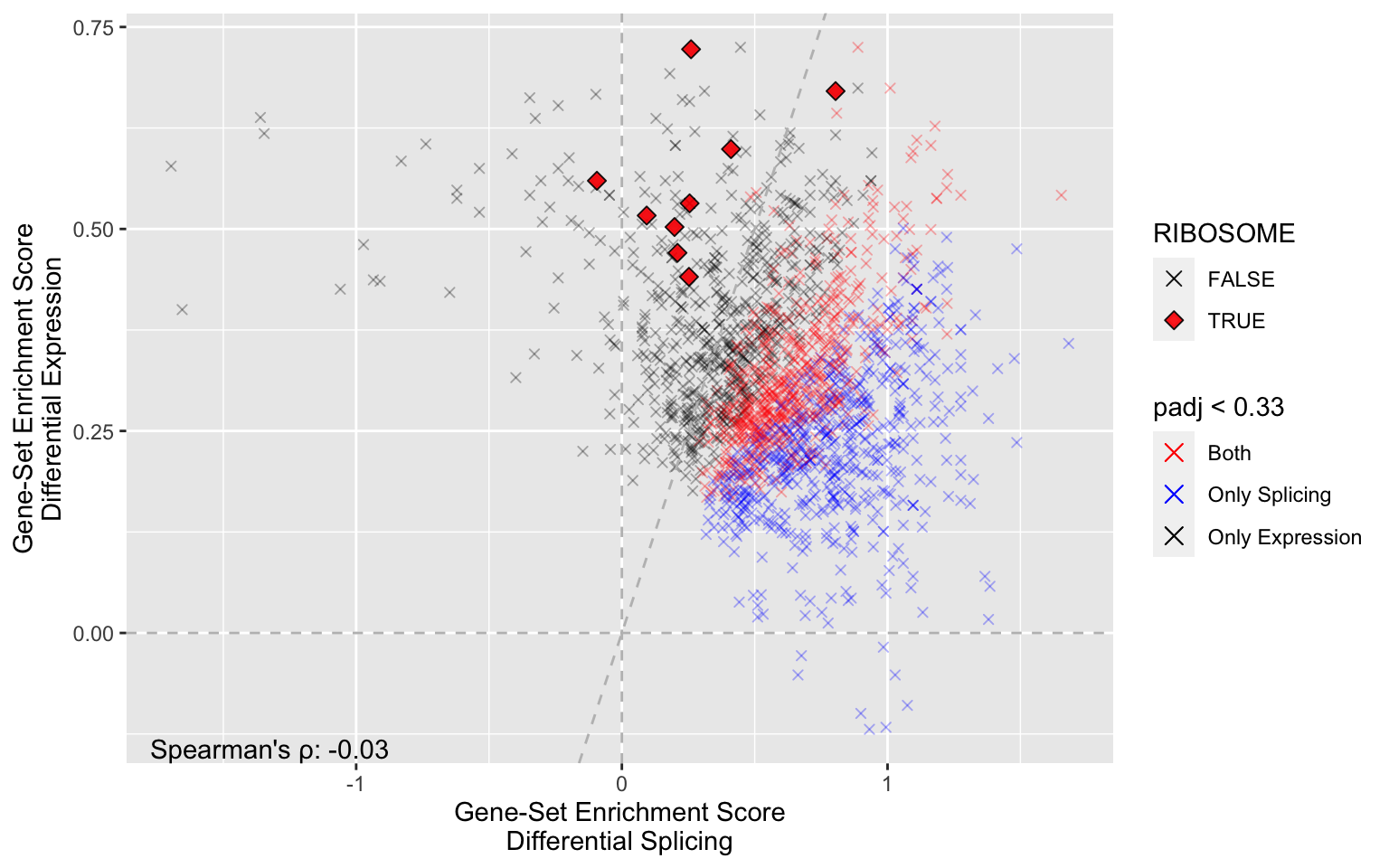
    pattern = "RIBOSOME", # Identify all gene sets about telomeres
    cutoff = 0.33, # Only include significant gene sets
    lines = TRUE, # Guide lines
    colors = c('red','blue','black')
)
 Ribosome is clearly mainly significant for DGE.
plot_ora(
    ora=cin_ora,
    plotly = FALSE,
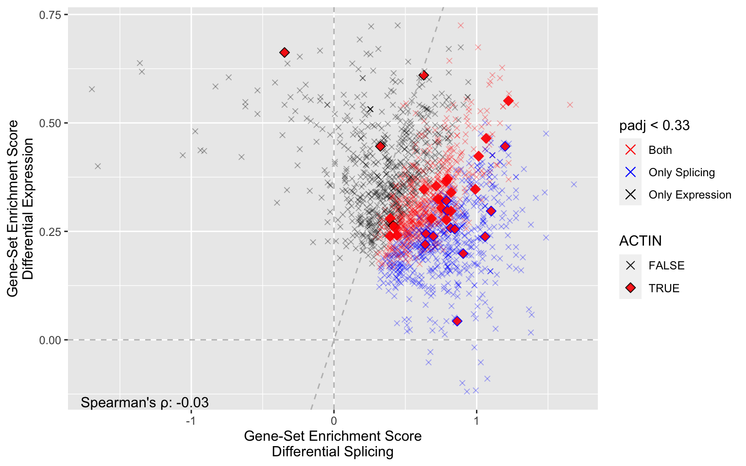
    pattern = "ACTIN", # Identify all gene sets about telomeres
    cutoff = 0.33, # Only include significant gene sets
    lines = TRUE, # Guide lines
    colors = c('red','blue','black')
)
Although many actin-related pathways are significant for both DGU and DGE more are DGU. Also, the enrichment among DGU is more pronounced (points are to the right of the diagonal line).
Lastly, note the low correlation suggesting an overall low similarity in biological signaling mediated through DGE and DGU.
Question: Try to make a hypothesis as to why this/these molecular functions might be important for cancer.
Answer:
- CELL_CYCLE: One of the main hallmarks of cancer - uncontrolled cell division.
- RIBOSOME: Many ribosomes are needed when cells are dividing (as indicated by increased cell cycle).
- ACTIN: Actin is involved in cell movement and thereby cancer invasion and metastasis.
Step 10: Critical self evaluation
Question: Take a moment to think about what potential problems there could be with this assignment. Are there any obvious things we have not taken into consideration?
Answer: The main problems are:
- More QC should have been done (clustering, outliers, etc)
- This is only a subset of the data (the real dataset has ~300 cancer samples)
- We do not take co-factors into account. How many of the effects are due to e.g. gender and age differences?
Step 11: Report result
Go to the blackboard and report one or more of the following:
- A keyword that showed a similar enrichment pattern in DGU and DGE
- A keyword that showed preferential regulation through DGU or DGE
Bonus Assignment
Use 'pairedGSEA' to analyze the other COAD cancer subtype (the one you did not analyze). Are the gene-sets similar or different between the subtypes and analysis types?

