Bayesian phylogenetics: checking convergence

This exercise is part of the course Computational Molecular Evolution (22115).

Check convergence using Tracer

In this exercise you will be briefly introduced to how to check if an MCMC run has converged using the program Tracer from the BEAST2 package. You will do this by re-examining the output from the Bayesian analysis you did in the week 9 exercise.

---

Question 1

Issue this command to start the Tracer program:

tracer

Now import the two MCMC sample files from the MrBayes run you did in week 9 for the hcvsmall data set:

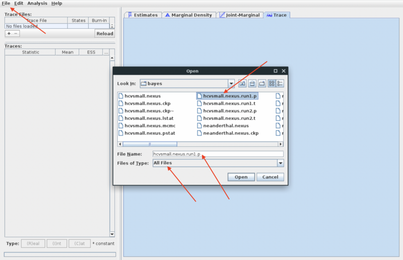
• File -> Import Trace File (or use the + under the trace file pane)
• In the import dialog: find the "bayes" directory and select "All files" under "files of type". This should give you a list of the output files from the MrBayes run
• Select the file "hcvsmall.nexus.run1.p" and open it.
• Repeat process for second log file (suffix ".run2.p")

You can now use Tracer to explore the results of the Bayesian analysis. The first thing you want to check is that the two independent runs have resulted in similar posteriors for the different parameters. This is investigated as follows:

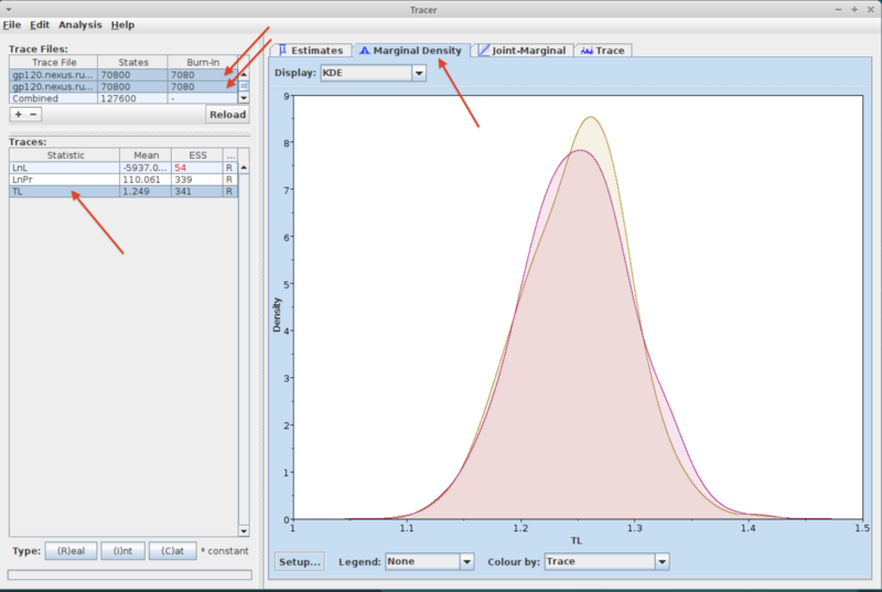
• Select both trace files by shift-clicking on their names in the "Trace files" pane (upper left of the Tracer window)
• Select the "Marginal Density" tab in the window on the right.
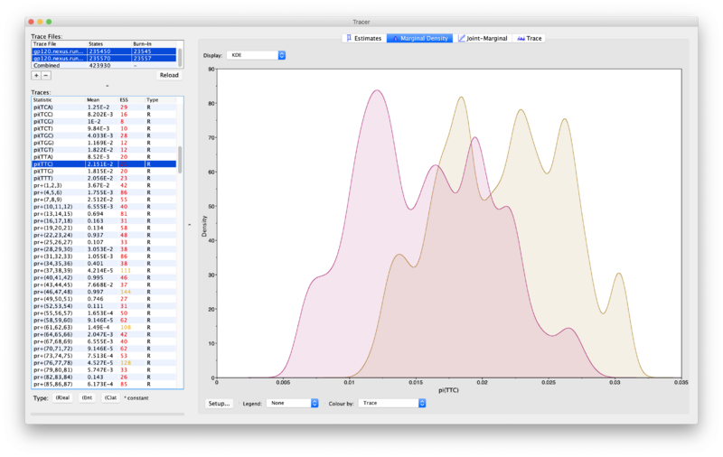
• Check different parameters by choosing them in the "Traces" pane on the left (while making sure you still have both trace files selected). This will show the two posteriors for the chosen parameter (see example below). If a run has converged then the two posteriors should mostly be placed right on top of each other.
• Note that Tracer by default uses a burnin of 10% of the total number of generations. You can change that by double-clicking in the Burn-in field of the trace file pane (you need to change it separately for each file). Typically we would use a burn-in of 25% or 50%.

• The plot below shows an example where convergence has not occurred yet:

Question: Take screen dumps of the marginal posterior plots for the following parameters and include them in your report: m{1} and piA{all}

---

Question 2

• Another thing to check is how the trace looks as a function of the iteration number: Optimally you would want a trace that looks like a "hairy caterpillar", with random jumps up and down on a mostly constant level (see example below).
• Select the "Trace" tab in the window on the right to see trace plots (still with one or both trace files selected in the Trace File pane).
• Related to this: The ESS column gives the "Effective Sample Size" for each parameter. As a rule of thumb we want this to be at least 200 (and Tracer flags smaller values by colouring the ESS values).
  • Briefly, the problem here is that consecutive samples from MCMC are correlated (they are not independent). This is due to the use of a Markov chain for sampling: the new position in parameter space depends on the previous location (and the proposal distribution).
  • The degree of non-indepence can be quantified by the auto-correlation for different lags: The autocorrelation for lag k is found by computing the Pearson correlation between all samples, and the samples k generations later.
  • Based on computation of auto-correlation at different lags ($k=[1,2,3,...]$) Tracer determines the Auto-Correlation Time (ACT), which is the number of generations in the MCMC chain that two samples have to be separated by for them to be uncorrelated. The ACT for a parameter can be seen in the Estimates tab in Tracer.
  • Tracer also estimates the Effective Sample Size (ESS), which is the number of independent samples that the trace is equivalent to. This is essentially the chain length (excluding the burn-in) divided by the ACT.
• Note how the highlighted parameter corresponding to the hairy caterpillar trace also has a high ESS in the example below.

• Trace plots where there are clearly visible dips and rises (see example below) indicates that there is auto correlation among the samples we have included - the samples are not independent of each other (and therefore provide less information about the posterior). This is referred to as "poor mixing". One solution to such a problem is to increase the number of iterations (and perhaps write samples less frequently). It might also be an indication that the model fits poorly, and that you could get a better convergence by changing the substitution model, or setting more informative priors.
• Note how the poorly mixing parameter in the example below also has a low ESS.

Question: Take screen dumps of the trace plots for the following parameters and include them in your report: m{1} and piA{all}. What is the ESS for these parameters?