IgraphIntro Ex v1

Introduction to working with networks in R

Exercise written by: Rasmus Wernersson and Lars Rønn Olsen

The purpose is to give a general introduction to the R packages igraph and ggraph, which we will be using for a large part of the course for:

1. Building and storing networks in R
2. Visualization / inspection of biological networks
3. Data integration of networks and supporting information

Working with TEXT files

As was the case in the prerequisite course Introduction to Bioinformatics (27611/27622) we will be working a lot with PLAIN TEXT files in this course, to import data into R. For this purpose you'll need a good TEXT EDITOR, that can save a file without a lot of formatting information. You can either use the built-in editor in RStudio or something like Sublime text or J edit

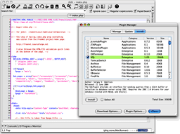
If you need a reminder on how to use text editors, you can briefly run through the old jEdit exercise.

Example: protein complexes

In the Systems Biology course we will be working a lot with protein-protein interaction data (physical interactions between proteins), and we'll start this exercise with a look at how we can represent a simple well-known protein complex in R, and how we can expand our analysis from here.

Structure of horse hemoglobin (from PDB) - the structure is a TETRAMER consisting of two ALPHA globins and two BETA globins.

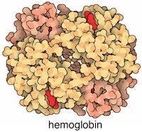
One of the simplest formats for storing graphs is using a two column data frame with connected proteins in each row (column names does not matter). For example, the physical interaction between ALPHA and BETA GLOBIN in the HEMOGLOBIN complex could be stated as:

hemoglobin <- data.frame(from = c("ALPHA_GLOBIN", "ALPHA_GLOBIN", "BETA_GLOBIN"), to = c("ALPHA_GLOBIN", "BETA_GLOBIN", "BETA_GLOBIN"))

Each of the ALPHA and the BETA globins also physically interacts with itself (see the structure for explanation).

igraph

igraph offers many ways to create a graph. The simplest one is the function make_empty_graph, but graphs can also be imported from and exported to a variety of file formats. The r.igraph website is a great introductory resource that you are encouraged to explore. The igraph package can do loads more than what is listed on their introductory website, and you are encouraged to use Google to find functions and examples for specialized tasks.

TASK: Make simple network in igraph

1. Login to the RStudio server.
2. Load the igraph package
3. Make an igraph object from the hemoglobin data frame using the graph_from_data_frame function (set "directed = FALSE" - we will explain why you should do this in detail throughout the course)
4. Plot the graph object using the base plot function (plot())

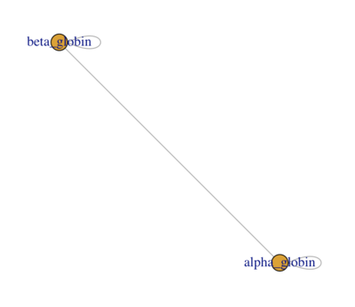
When you're done you should have a network that looks similar to the screenshot below:

• Make sure you understand what the NODES (the circles) and the EDGES (the lines) represent: what is the BIOLOGICAL interpretation of the network?

DNA Polymerase Delta

Schematic overview of the Eukaryotics replication machinery - notice Polymerase Delta working on the lower DNA strand. Source: Wikipedia

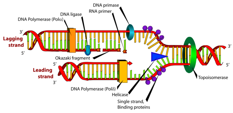
Before we move on to the more advanced visualization feature of ggraph, we'll introduce a slightly more complex network which we can expand upon as we go along: DNA Polymerase Delta (Pol δ). Pol δ has "proofreading" fuctionality (3'→5' exonuclease activity) and consist of the "proliferating cell nuclear antigen" (PCNA), a multi-subunint complex named "replication factor C" and the polymerase subunit itself, which consists of four proteins: POLD1, POLD2, POLD3 and POLD4.

Pol δ network

We will start out with having a look at the polymerase sub-unit. Since we want to expand the network and add in more information as we go along, we choose to map the proteins to actual UniProt identifiers, which will make it easy to look up additional information as we go along:

Gene   Protein 
----   -------
POLD1  DPOD1_HUMAN
POLD2  DPOD2_HUMAN
POLD3  DPOD3_HUMAN
POLD4  DPOD4_HUMAN

UniProt links (for optional browsing):

• http://www.uniprot.org/uniprot/DPOD1_HUMAN
• http://www.uniprot.org/uniprot/DPOD2_HUMAN
• http://www.uniprot.org/uniprot/DPOD3_HUMAN
• http://www.uniprot.org/uniprot/DPOD4_HUMAN

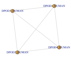
TASK: create data frame for the polymerase sub-unit interactions:

• The subunit is a tetramer consisting of one of each protein.
• Each protein interacts with all other proteins.
• Your igraph network should look similar (have the same topology) as the network shown here.

Pol δ node attributes

In order to visualize graph to understand and communicate their properties, we can add attributes to both the nodes and edges of the graph.

For example if you follow the UniProt links above, you can read a wealth of information about the names, descriptions, biological function and much more for each of the proteins.

IMPORTANT NOTE: in graph theory, nodes can also be referred to as "vertices" (singular: vertex) and this is the convention in igraph.

Adding attributes to igraph object

To add node attributes to an igraph object, please see that the graph_from_data_frame function has a variable "vertices" which allows you to add node attributes in the form of a data frame when you build the igraph object. Adjusting and retrieving attributes of an igraph object once it is made, can be done using the functions V() (to add vertex attributes) and E() (to add edge attributes). Please see the igraph documentation for information on how this works.

In other words, the simplest way to add node attributes is to create a node attribute data frame. The first column of the data frame is assumed to contain symbolic vertex names, this will be added to the graphs as the ‘name’ vertex attribute. Other columns will be added as additional vertex attributes.

For example:

UniProtId GeneID  Catalytic Description AA
DPOD1_HUMAN PolD1 yes DNA polymerase delta catalytic subunit 1009
DPOD2_HUMAN PolD2 no  DNA polymerase delta subunit 2 469
DPOD3_HUMAN PolD3 no  DNA polymerase delta subunit 3 466
DPOD4_HUMAN PolD4 no  DNA polymerase delta subunit 4 107

As can be seen from the example, 4 categories of information have been added, and each line contains information related to a single protein. The node attributes will be assigned the column names, such that for example "Description" can be retrieved or edited using V(g)$Description. "AA" refers to the length of the amino acid sequence of the protein.

TASK: Import the node attribute table into a new pol delta igraph object

1. Make a data frame of the node attribute table above (do this manually for now - we will later learn how upload and read data into RStudio)
2. Make a new igraph object of the pol delta network and include the node attributes
3. Check that this worked using the function "V()"

Visualizing the graph using ggraph

ggraph (pronounced "g-giraph) is an extension of ggplot2 aimed at supporting relational data structures such as networks, graphs, and trees. If you have not yet worked with ggplot2, or feel like you need a reminder of how it works, here is a good primer. This web site gives an excellent overview of the functionalities of ggraph and serves as a great reference. Take a moment to browse ggraph's functionalities.

TASK - use the node annotations for customizing visualization

1. Plot the pol delta complex using ggraph and the default layout

way to visualize protein-protein interactions?

1. Label:
   • Modify it to show the GeneIDs (you will have to find out how yourself - HINT: try to search google for "ggraph node labels")
2. Fill Color:
   • Color the nodes based on the "Catalytic" variable in the
3. Node size:
   • Make the size of the nodes correspond to the length of the amino acid sequence

Report: Q1: Paste a screenshot of your nicely decorated network into you report

Extended Pol δ network

For the final part of the exercise we'll be working with set of experimental data centered around the Pol δ complex. Later in the course we will learn a lot of details about how such experimental data is generated, what strengths and weaknesses the different methods have, and how we can address the noise in the data.

For now it sufficient to note the following:

• The experiment has detected proteins that physically interacts with the PolD1-PolD4 complex we have just worked with.
• Both stable and transient interactions have been identified.
• The experiment shows some of the most likely interactions - additional experiments may find more.
• The data may contain false positive (proteins indicated to interact, while that is not true under real biological conditions).

Network and layout

ggraph visualization with default (stress) layout. Could this be improved?

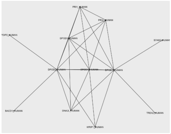
poldelta_extented_interactions <- data.frame(from = c("DPOD1_HUMAN", "DPOD1_HUMAN", "DPOD1_HUMAN", "DPOD1_HUMAN", "DPOD1_HUMAN", "DPOD1_HUMAN", "DPOD1_HUMAN", "DPOD1_HUMAN", "DPOD1_HUMAN", "DPOD2_HUMAN", "DPOD2_HUMAN", "DPOD2_HUMAN", "DPOD2_HUMAN", "DPOD2_HUMAN", "DPOD2_HUMAN", "DPOD2_HUMAN", "DPOD2_HUMAN", "DPOD3_HUMAN", "DPOD3_HUMAN", "DPOD3_HUMAN", "DPOD3_HUMAN", "DPOD4_HUMAN", "DPOD4_HUMAN", "DPOD4_HUMAN", "DPOD4_HUMAN", "PRI1_HUMAN", "WRIP1_HUMAN"), to = c("DPOD2_HUMAN", "DPOD3_HUMAN", "DPOD4_HUMAN", "S7A6O_HUMAN", "TREX2_HUMAN", "DNA2L_HUMAN", "PRI1_HUMAN", "PRI2_HUMAN", "WRIP1_HUMAN", "DPOD3_HUMAN", "DPOD4_HUMAN", "PDIP2_HUMAN", "BACD1_HUMAN", "WRIP1_HUMAN", "DNA2L_HUMAN", "PRI1_HUMAN", "PRI2_HUMAN", "DPOD4_HUMAN", "DNA2L_HUMAN", "PRI1_HUMAN", "PRI2_HUMAN", "DNA2L_HUMAN", "PRI1_HUMAN", "PRI2_HUMAN", "WRIP1_HUMAN", "PRI2_HUMAN", "WRIP1_HUMAN"))

TASK - import the network

TASK - find a good network layout

1. Play around with a few other layouts. Think about whether they are good or bad for visualizing a protein-protein interactions (for example, do you think that the "linear" layout would be a good visualization for this topology?)

Collecting node attributes

The next step in the network analysis, is to gather a set of useful information about the protein in the network, that can help guide our understanding of the biology behind the network. This information gathering will have two goals:

• To collect NODE ATTRIBUTE information useful for visualization of the network.
• To get an initial understanding of what the roles of the individual proteins may be:
  • E.g. biological process, cellular compartment, description, notes about function etc.

Node attributes in the process of being collected in an Excel sheet

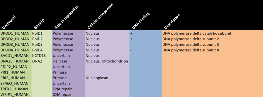
There are a number of (semi) automatic ways to gather such data, but since we're working with a small network here, it's feasible to manually gather the data from a well respected data source such as UniProt, and keeping track of it in a spreadsheet you can then load into R, or you can record the info directly into a data frame, if you prefer.

TASK - gather protein information

• We have prepared a partially filled out Excel sheet (see the screenshot above) which will form the basis for the data gathering.
  • Download the Excel sheet from HERE: PolDelta_Extended_NodeAttribute_Worksheet_2020.xlsx
• Use the UniProt links below to find the following information (ask the instructor for help if you get stuck):
  • Description
  • Gene name
  • Is the protein known to bind DNA? (+/-)
  • Which cellular compartments is the protein known to be located in?
• For the proteins marked as UNCERTAIN with regard to role in replication:
  • Can you find any additional information that indicates that they are actually working together with the other proteins in the network?
  • (Note: some of them may be in the network due to experimental error.)
• Bonus question: WRIP1_HUMAN has an interaction with itself. Is there a good explanation for this?

UniProt links:

• http://www.uniprot.org/uniprot/DPOD1_HUMAN
• http://www.uniprot.org/uniprot/DPOD2_HUMAN
• http://www.uniprot.org/uniprot/DPOD3_HUMAN
• http://www.uniprot.org/uniprot/DPOD4_HUMAN
• http://www.uniprot.org/uniprot/BACD1_HUMAN
• http://www.uniprot.org/uniprot/DNA2_HUMAN
• http://www.uniprot.org/uniprot/PDIP2_HUMAN
• http://www.uniprot.org/uniprot/PRI1_HUMAN
• http://www.uniprot.org/uniprot/PRI2_HUMAN
• http://www.uniprot.org/uniprot/S7A6O_HUMAN
• http://www.uniprot.org/uniprot/TREX2_HUMAN
• http://www.uniprot.org/uniprot/WRIP1_HUMAN

Report: Q2: paste a screenshot of the final data frame into a your report.

Visualizing node attributes

The next step is to make an igraph object of the interactions and the node attributes you collected.

TASK - visualize the Node attributes

• Node label - use GeneID
• Node color - color based on "Role in replication" (invent your own coloring scheme)
• Node shape - pick two shapes to represent whether the protein is known to bind to DNA

Report: Q3: Answer the following question: Does it make sense that some of the proteins are not annotated to bind DNA yet are supposed to have a role in DNA replication? (For example DPOD3_HUMAN and DPOD4_HUMAN)

Edge attributes

As the final part of the exercise we'll include edge attributes to the igraph object. This can be done simply by including additional columns in the interaction data frame. By default, the graph_from_data_frame() function reads the first two columns as node names, and all following columns as attributes of the edges between the nodes.

Each edge in the Pol δ network represents a protein-protein interaction determined experimentally. A number of different pieces of information could potentially be associated with each interaction:

• Experimental method used.
• Whether the interaction is stable or transient.
• How much experimental support is there for the interactions (e.g. a single experiment, 3 experiments or 100+ experiments).

Below are the confidence scores of all the interactions in the extended pol delta network. Simply add the vector below to the poldelta_extented_interactions data frame.

c(1.00, 1.00, 1.00, 0.18, 1.00, 1.00, 1.00, 1.00, 0.52, 1.00, 1.00, 1.00, 1.00, 0.54, 1.00, 1.00, 1.00, 1.00, 1.00, 1.00, 1.00, 1.00, 1.00, 1.00, 0.57, 1.00, 0.65)

You may consider the following interpretation of the score:

0.0 - 0.3 : poor experimental support
0.3 - 0.9 : "good enough" experimental support
0.9 - 1.0 : excellent experimental support

TASK - import and visualize network

• Make an igraph object with the interactions, edge attributes, and node attributes
• Visualize the network with ggraph, adding some formatting of the edges continuously by the confidence score (color, width, or transparency are good options)
• Make a discrete vector based on the three categories above, and add reload the igraph object. Make three different colors, widths, line types, or whatever else you can come up with to make a visually pleasing and informative visualization.

Which do you prefer - continuous or discrete visualization of line colors?

Report: Q4: Document your network(s) by pasting screenshots into your report.

FINAL QUESTION - Re-evaluate the three "uncertain" proteins (BACD1_HUMAN, PDIP2_HUMAN, S7A6O_HUMAN):

• Consider the following points and make a conclusion based on the combined evidence on which of the three proteins are likely to be true interaction partners:
  • The proteins they are interacting with.
  • The experimental support for the interactions.
  • Any biological information (any hints, basically) you may have picked up from skimming through the UniProt pages for each of the three proteins.

Report: Q5: Briefly describe your consideration, findings, and potential updates.