QuantitativeMetagenomics
Overview
If you need to use metagenomics for your final project, we have a more thorough workflow that you will need to use [here].
Since metagenomics data is often very large, it requires a lot of computational resources and time, we have cheated a little bit and prepared some data for you in advance!
In this exercise we have done the assembly and counting across a cohort of hundreds of human fecal samples in advance and in addition provide the gene-wise taxonomy and the BMI of the human donors. From this data we shall estimate the species richness, diversity and look at the effect of downsizing. Furthermore we shall see if we can identify any differences between the microbiome of lean and obese.
Becoming a pirate
This exercise uses R either locally (install RStudio on your own machine) or on the server by typing
R
First, IF you are running RStudio locally you will need to install a package called "vegan"
install.packages("vegan")
Now, let’s load the "vegan" package and thereafter load the read count data from a series of stool samples.
library("vegan")
load(url("http://teaching.healthtech.dtu.dk/material/22126/Counts_NGS.RData"))
head(Counts)
str(Counts)
Q1. How many samples do we have and how many genes?
The different samples may have been sequenced to different depths. Try to count the reads per sample
sampleDepth<-(colSums(Counts))
hist(sampleDepth, breaks=100, ylab="Number of samples", xlab="Number of reads", main="Sample depth")
range(sampleDepth)
Q2. Whats the sample depth range?
Species
Lets get the genes associated to species. Here is the gene-wise species taxonomy
load(url("http://teaching.healthtech.dtu.dk/material/22126//taxonomy_species.RData"))
head(taxonomy_species)
We then combine (by summing) the read counts pr. gene to read counts per species.
taxCounts<-apply(Counts, 2, tapply, INDEX=taxonomy_species, sum)
Try looking at the taxCounts matrix
str(taxCounts)
head(taxCounts)
Q3. How many species are there in total?
Richness and Diversity
What is the species richness and diversity (Shannon) for the different samples.
Q4. What does a high Shannon diversity index mean?
OK, lets see it for our samples
species_richness<-(colSums(taxCounts>0))
names(species_richness)<-NULL
require(vegan)
speciesDiversity<-diversity(t(taxCounts), index = "shannon")
names(speciesDiversity)<-NULL
par(mfrow=c(1,1))
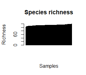
barplot(sort(species_richness), las=3, main="Species richness", xlab="Samples", ylab="Richness")
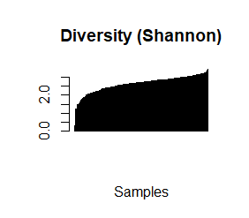
barplot(sort(speciesDiversity), xlab="Samples", las=3, main="Diversity (Shannon)")
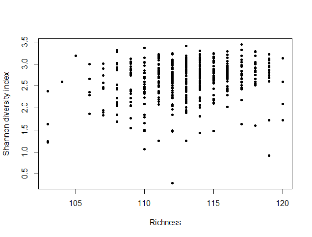
plot(species_richness,speciesDiversity,xlab="Richness", ylab="Shannon diversity index")
Each samples or persons richness and diversity is shown and the third plot shows each sample/persons richness & diversity as a dot.
Downsizing or rarefying
But this was on the raw count data with different sampling depth (number of counts) per sample. We should downsize so that we get fair comparisons.
First suggest the number of reads we should sample per sample for the downsizing [target]. If we chose a low target we will loose abundance resolution and detection sensitivity. If we chose it higher we will loose samples.
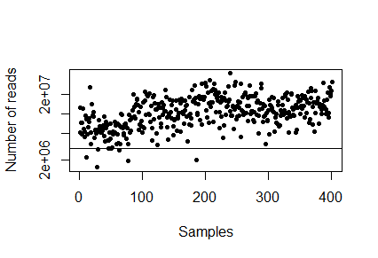
> plot(sampleDepth, pch=20, log="y", xlab="Samples", ylab="Number of reads")
There is no right answer (but there are less good suggestions). Insert the number you want to downsize to below and plot it again - the samples above the horizontal line we will keep and the samples below the line we will throw out.
> downsizeTarget <- INSERT NUMBER
> plot(sampleDepth, pch=20, log="y", xlab="Samples", ylab="Number of reads"); abline(h=downsizeTarget)
Q5. Which threshold did you chose and why? How many samples did you loose?
OK lets downsize
> dz_Counts<-round(t(t(Counts)*downsizeTarget/sampleDepth))
> weak_samples<-sampleDepth<downsizeTarget
> dz_Counts[,weak_samples]<-NA # samples that did not make the cut
This is a quick and dirty downsizing (ideally one resampled the reads to a given depth, but that will take days) Count the species again, now on the downsized data.
dz_taxCounts<-apply(dz_Counts, 2, tapply, INDEX=taxonomy_species, sum); gc()
And the richness and diversity again, now on downsized data
> dz_species_richness<-(colSums(dz_taxCounts>0))
> names(dz_species_richness)<-NULL
> require(vegan)
> dz_speciesDiversity<-diversity(t(dz_taxCounts), index = "shannon")
> dz_speciesDiversity[weak_samples]<-NA
> names(dz_speciesDiversity)<-NULL
Now plot the richness and diversity with downsized data
> par(mfrow=c(1,1), pch=1)
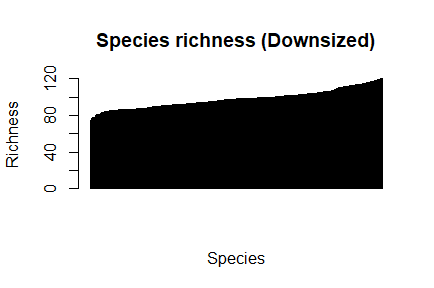
> barplot(sort(dz_species_richness), las=3, main="Species richness (Downsized)", xlab="Species", ylab="Richness")
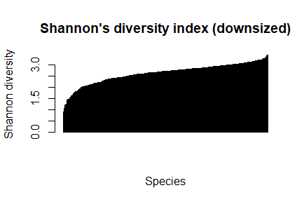
barplot(sort(dz_speciesDiversity), las=3,main="Shannon's diversity index (downsized)", xlab="Species", ylab="Shannon diversity")
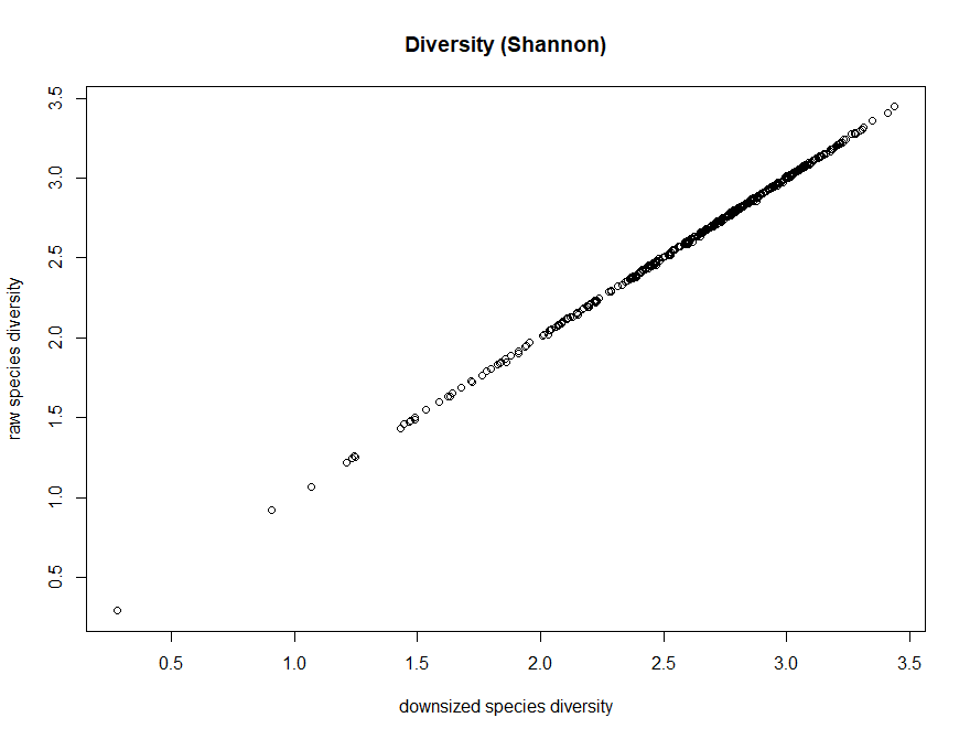
And compare to the raw data
> plot(dz_species_richness,species_richness, xlab="downsized richness", ylab="raw richness", main="Richness")
> plot(dz_speciesDiversity,speciesDiversity,xlab="downsized species diversity", ylab="raw species diversity",main="Diversity (Shannon)")
Q6. What is the effect on the downsizing on richness
Q7. What is the effect on the downsizing on diversity (shannon)
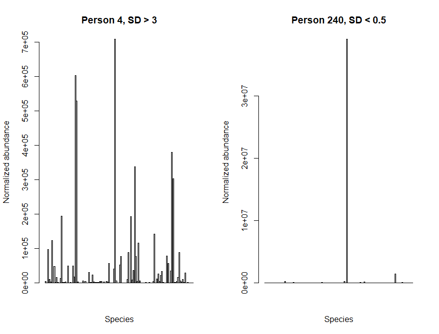
Lets plot the abundance of each species in a sample with low diversity and a sample with high diversity. You should be able to see a clear difference between the two samples!
> par(mfrow=c(1,2))
> barplot(taxCounts[,4], main="Person 4, SD > 3", xaxt="n", xlab="Species", ylab="Normalized abundance")
> barplot(taxCounts[,240], main="Person 240, SD < 0.5", xaxt="n", xlab="Species", ylab="Normalized abundance")
> par(mfrow=c(1,1))
Comparisons
Now lets see if there is a difference between the microbiome of lean and obese humans. But first load some sample more information: BMI and Class.
> load(url("http://teaching.healthtech.dtu.dk/material/22126/BMI.RData"))
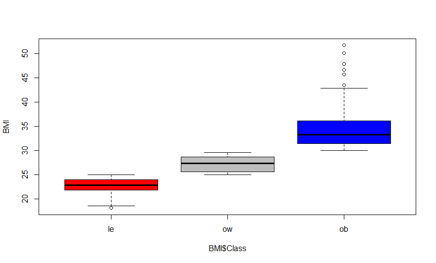
> boxplot(BMI$BMI.kg.m2 ~ BMI$Class, col=c("red", "gray","blue"), ylab="BMI")
Class are: le = Lean; ow = Overweight; ob = Obese
First let us see if the abundance of E. coli differs between obese and lean individuals using a Wilcoxon rank sum test (look for the p-value in the output), also lets get the mean abundance of E. coli in the tree groups :
> wilcox.test(x=dz_taxCounts["Escherichia coli",BMI$Classification=="ob"], y=dz_taxCounts["Escherichia coli",BMI$Classification=="le"] )
> tapply(dz_taxCounts["Escherichia coli",], BMI$Classification, mean, na.rm=TRUE)
Q8. Is there any significant difference in abundance of E. coli between the different BMI groups?
Let's test all species correcting for multiple testing using Benjamini-Hochberg (False Discovery Rate) (we are testing 120 species) and plot them:
> pval<-apply(dz_taxCounts, 1, function(V){wilcox.test(x=V[BMI$Classification=="ob"],y=V[BMI$Classification=="le"])$p.value})
> Abundance_ratio<-log2(apply(dz_taxCounts, 1,function(V){mean(x=V[BMI$Classification=="ob"], na.rm=TRUE)/mean(V[BMI$Classification=="le"], na.rm=TRUE)}))
> pval.adjust = p.adjust(pval, method="BH")
> plot(sort(pval.adjust), log="y", pch=16, xlab="Species", ylab="p-values")
> abline(h=0.05, col="grey", lty=2)
Q9. How many species are significant with an false discovery rate < 0.05?
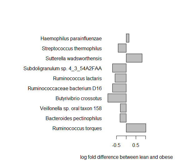
Let us look at the top 10 most significant species abundance.
> o<-order(pval)
> BMIstat<-data.frame(pval,pval.adjust, Abundance_ratio)[o,]
> BMIstat[1:10,]
> par(mar=c(5,18,5,5))
> barplot(BMIstat[1:10,3], names.arg=rownames(BMIstat)[1:10], las=1,xlab="log fold difference between lean and obese", horiz=TRUE)
Q10. Can you see any differences in the abundances - which species have large differences, what are their p-values?
Q11. What type of bacteria is the most significant one? [try google]
Beta-diversity and PCA
Plot the Bray-curtis distance between samples as a heatmap.
library(RColorBrewer)
library(gplots)
vdist = as.matrix(vegdist(t(taxCounts)))
rownames(vdist) = colnames(vdist)
hmcol = colorRampPalette(brewer.pal(9, "GnBu"))(100)
heatmap.2(vdist, trace='none', col=rev(hmcol))
Q12. Can you see some clusters of samples?
Finally for the PCA:
> my.rda <- rda(t(taxCounts))
> biplot(my.rda, display = c("sites", "species"), type = c("text", "points"))
Q13. Can you see which species that seems to be driving the differences between the samples?
Statistically modelling the variance using DESeq2
Now, we will see the power of statistically modelling the variance instead of downsizing.
> if (!requireNamespace("BiocManager", quietly = TRUE))
> install.packages("BiocManager")
> BiocManager::install("DESeq2")
> library(DESeq2)
> cts <- taxCounts
> coldata = BMI[,1]
> coldata = matrix(NA, nrow=nrow(BMI), ncol=1)
> coldata[,1] = as.vector(BMI[,1])
> rownames(coldata) = rownames(BMI)
> colnames(coldata) = "BMI"
Take a look at coldata
coldata
Make sure that all individuals are in our coldata (information) and also in the data is true
all(rownames(coldata) == colnames(cts))
Load data into DESeq format, perform statistical analysis and get results
> dds <- DESeqDataSetFromMatrix(countData = cts, colData = coldata, design = ~ BMI)
> dds <- DESeq(dds)
> res <- results(dds)
> res
Order the results according to the adjusted p-value and show the most significant
> resOrdered <- res[order(res$pvalue),]
> head(resOrdered)
Q14. which are the most significant species (google)? Is there an overlap between these and using downsizing+wilcoxon test (what you did above)?
Please find answers here
